Climate Warming Pattern Recognition from CMIP6 Simulations
A scalable analysis of CMIP6 climate simulations that measures how the annual distribution of temperatures is changing across the globe, identifies regions with similar warming patterns, and examines how these patterns shift over the long term.
The problem
Climate change is often summarized by a single number, such as the rise in global mean temperature. However, warming varies from region to region, and it also varies within each location’s temperature distribution: the coldest periods of the year may warm at a different rate than the warmest ones. These differences matter because many impacts, such as heat stress, frost, and ice loss, depend on the extremes rather than on the average.
The goal: measure how the annual distribution of temperatures is changing at every location on Earth, and identify regions that share similar warming patterns.
Data
CMIP6 · NOAA-GFDL GFDL-ESM4 climate model
The data come from simulations of the GFDL-ESM4 model in the Coupled Model Intercomparison Project Phase 6 (CMIP6). The analysis uses the historical simulation for 1948–2014 and the future projection for 2015–2100 under SSP1-2.6, a low-emissions scenario. Both are read directly from the Pangeo cloud catalog of CMIP6 data.
Approach
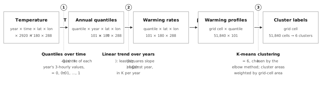
A three-step pipeline was built to turn high-frequency temperature data into a warming profile for each location and then group locations with similar profiles. The same pipeline is applied separately to the historical and future periods to identify long-term climate shifts across the globe.
1. Annual temperature distributions
For each grid cell and year, the empirical distribution of 3-hourly temperatures is characterized by 101 quantiles, spanning the coldest to the warmest conditions of the year.
2. Warming profiles
The warming rate of each quantile is estimated as the slope of a least-squares linear trend across years, in kelvin per year. The resulting 101 rates constitute the warming profile of each grid cell.
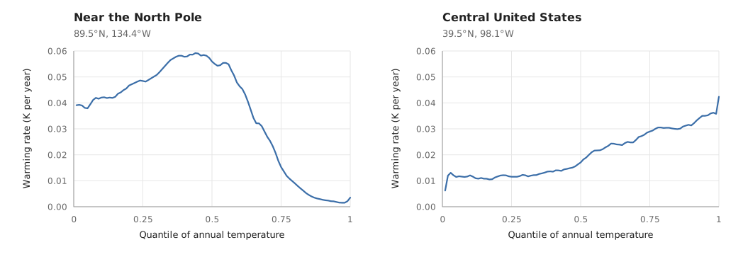
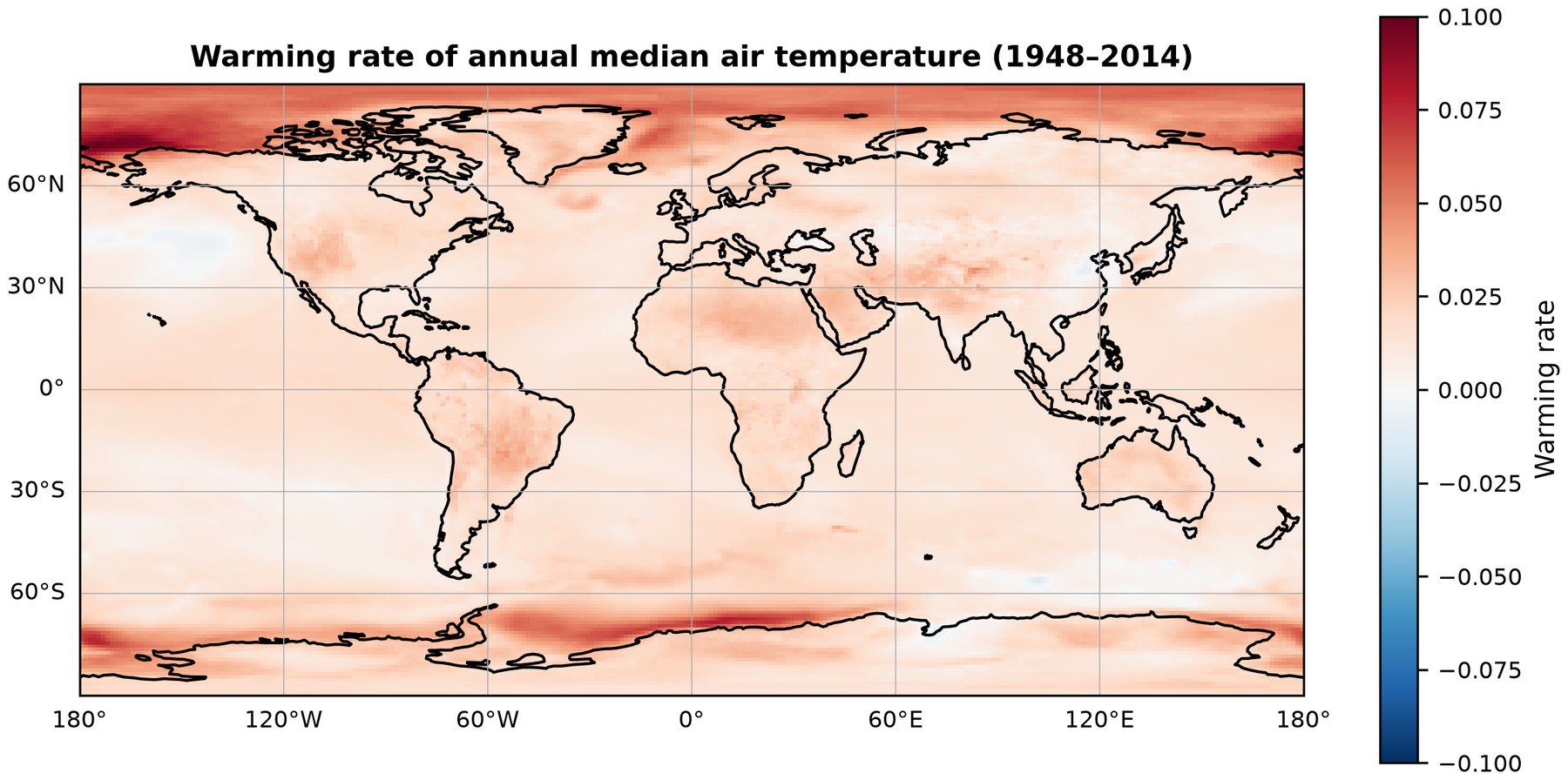
Mapping the warming rate of a single quantile shows the spatial pattern of change in one part of the distribution; the warming profile integrates all 101 quantiles at each location.
3. Warming pattern recognition
Grid cells are partitioned into k clusters based on their warming profiles, independent of geographic location, to identify regions that share similar warming patterns. The value of k is determined using the elbow method.
Scalable processing
Given the volume of the data, the pipeline relies on xarray and Dask for lazy, chunked computation, reading data directly from cloud storage without loading the full dataset into memory.
Results
- Fastest historical warming near the poles. From 1948 to 2014, the median temperature warmed fastest over the Arctic Ocean and along parts of the Antarctic coast.
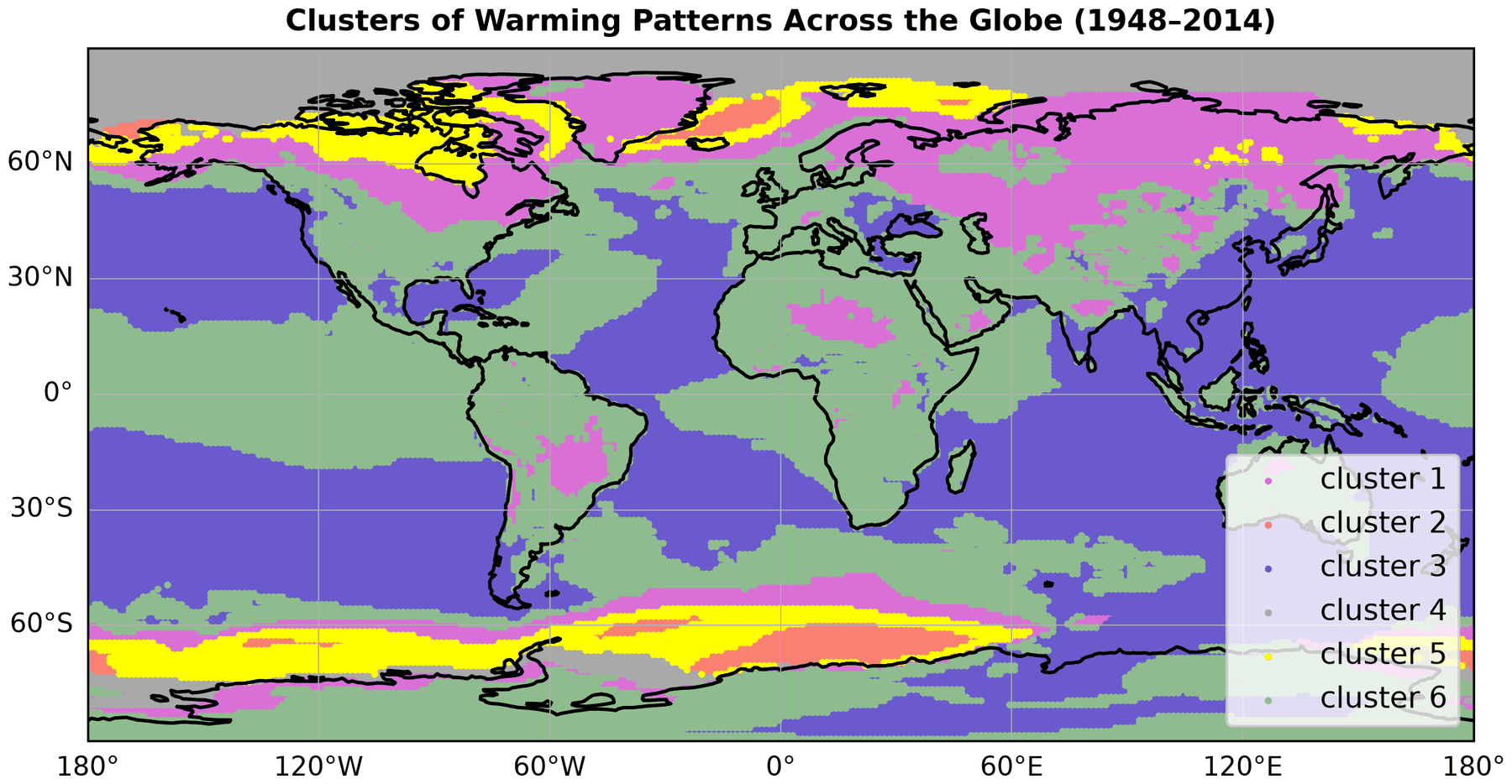
- Two dominant patterns. In the historical period, two patterns cover about 83% of the Earth’s surface. The other four are found mostly at high latitudes.
- Rapid warming of cold extremes. In the smallest historical pattern, covering about 1% of the surface east of Greenland and along parts of the Antarctic coast, the coldest periods of the year warmed several times faster than the warmest.
- Slower projected warming, fastest in the Arctic. Projected median warming for 2015–2100 is slower than in the historical period across most of the globe and fastest over the Arctic Ocean north of Alaska and eastern Siberia.
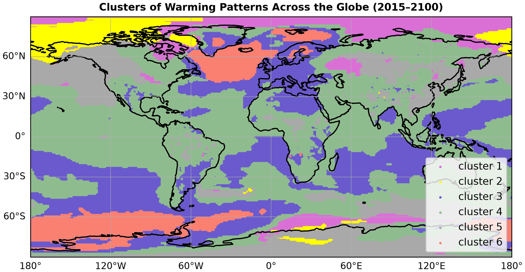
- Regional instead of polar patterns. The ring-like polar patterns of the historical period break up into regional ones. One pattern covers about half of the Earth’s surface, and areas with little or no warming, south of Greenland and off West Antarctica, form their own pattern.
The top image shows the historical patterns; the map below shows the projected patterns for 2015–2100.
Methods & tools
Climate data analysis · statistical trend analysis · pattern recognition · geospatial analysis · large-scale data processing · Python · xarray · Dask · scikit-learn